Interaction Effects in Regression: When One Predictor's Effect Depends on Another

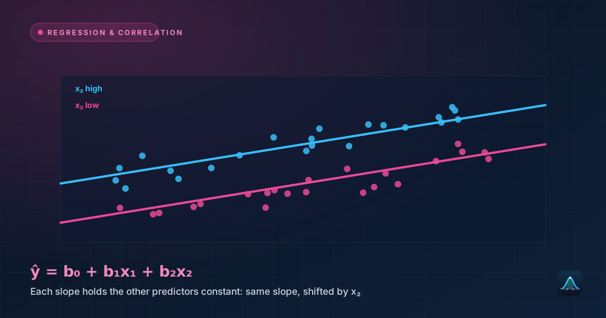
A standard multiple regression model assumes each predictor has one fixed effect on the outcome, whatever values the other predictors take. Often that is too simple. A training programme might help beginners far more than experts; a price cut might lift sales strongly in one region and barely at all in another. When the effect of one predictor genuinely depends on the level of another, the model needs an interaction term — a product of the two predictors — to capture it.

Why Parallel Lines Are Not Always Enough

In dummy variable regression, adding a 0/1 group indicator to a model with a numeric predictor produces two parallel lines: the groups can start at different heights, but the slope is identical for both. That is an assumption, not a discovery. If one group's outcome really does grow faster with the numeric predictor than the other's, forcing equal slopes distorts the fit for both groups.

The fix is to add a third term, the product of the numeric predictor and the dummy variable. For a numeric predictor x and a 0/1 group indicator D, the model becomes:

For the baseline group (D = 0), the last two terms vanish and the line is simply ŷ = b₀ + b₁x. For the other group (D = 1), the line becomes ŷ = (b₀ + b₂) + (b₁ + b₃)x. The coefficient b₂ therefore shifts the intercept, and b₃ shifts the slope. The interaction coefficient b₃ is precisely the difference in slopes between the two groups.

Worked Example

Problem: A company records years of experience and salary for four Sales employees and four Engineering employees. Sales is the baseline (D = 0); Engineering is coded D = 1.

Experience (years)	1	3	5	7
Sales salary	$43,000	$45,000	$49,000	$55,000
Engineering salary	$51,000	$59,000	$66,000	$72,000

Step 1 — Fit each group's own line. Fitting the model with the interaction term is equivalent to fitting a separate least-squares line within each group, using the method from simple linear regression. Both groups have experience values of 1, 3, 5, 7, so x̄ = 4 and Sxx = 20 for each.

For Sales, the mean salary is $48,000 and Sxy = 40 (in thousands of dollars), so the slope is 40 ÷ 20 = $2,000 per year and the intercept is 48,000 − 2,000(4) = $40,000.

For Engineering, the mean salary is $62,000 and Sxy = 70 (in thousands), so the slope is 70 ÷ 20 = $3,500 per year and the intercept is 62,000 − 3,500(4) = $48,000.

Step 2 — Translate into the interaction model. The baseline group's line supplies b₀ = 40,000 and b₁ = 2,000. The intercept difference gives b₂ = 48,000 − 40,000 = 8,000, and the slope difference gives b₃ = 3,500 − 2,000 = 1,500. The full fitted model is:

Step 3 — Read what it says. The predicted salary gap between Engineering and Sales is no longer a fixed number; it grows with experience:

Experience	Sales predicted	Engineering predicted	Gap
1 year	$42,000	$51,500	$9,500
3 years	$46,000	$58,500	$12,500
5 years	$50,000	$65,500	$15,500
7 years	$54,000	$72,500	$18,500

The gap at any experience level x is 8,000 + 1,500x. Each extra year of experience widens it by $1,500 — that is exactly what the interaction coefficient means.

Reading Every Coefficient Correctly

Once an interaction is in the model, the other coefficients change meaning, and this is where most misreadings happen.

• b₁ = 2,000 is the slope of experience for the baseline group only (Sales). It is not "the effect of experience" in general; Engineering's slope is b₁ + b₃ = 3,500.
• b₂ = 8,000 is the Engineering–Sales gap at zero years of experience, because that is the only point where the interaction term is zero. It is not an average gap across the data.
• b₃ = 1,500 is how much steeper Engineering's slope is than Sales' slope.

Testing Whether the Interaction Is Real

The eight points do not lie perfectly on the two lines; the residuals are ±1 (thousand) for Sales and ±0.5 for Engineering, giving a residual sum of squares of 4(1) + 4(0.25) = 5 on 8 − 4 = 4 degrees of freedom, so the mean squared error is 5 ÷ 4 = 1.25. The standard error of the slope difference is √(1.25 × (1/20 + 1/20)) = √0.125 ≈ 0.354, or about $354. The test statistic for b₃ is:

The difference in slopes is statistically distinguishable from zero. The same conclusion appears when comparing the two models directly. A model forced to have parallel lines fits these data with a residual sum of squares of 27.5, against 5 for the interaction model. The F statistic for adding the interaction term is (27.5 − 5) ÷ (5 ÷ 4) = 18.0, which equals t² and gives the same p-value — the same partial F-test logic used for comparing nested regression models. R² rises from 0.962 to 0.993, a modest-looking jump that nonetheless represents the difference between an adequate fit and a correct description of the pattern. The parallel-lines model would also give misleading answers: it would claim a constant gap of $14,000, overstating the gap for junior staff and understating it for senior ones.

Two Numeric Predictors

Interactions are not limited to a dummy variable. With two numeric predictors x and z, the model ŷ = b₀ + b₁x + b₂z + b₃(xz) says the effect of x on y is b₁ + b₃z: it changes continuously as z changes. When both predictors are centered first (each has its own mean subtracted), b₁ becomes the effect of x at the average value of z rather than at z = 0, which is usually a more meaningful reading, and centering also reduces the correlation between the product term and its components, easing the multicollinearity concerns discussed in multiple regression.

Real-World Uses

Medicine and drug response: a treatment's benefit may depend on a patient characteristic such as age or baseline severity, so a treatment × severity interaction captures who benefits most.

Marketing and pricing: the effect of a promotion on sales often differs by region or customer segment, which a promotion × segment interaction models directly.

Education research: the gain from a teaching method may differ between students with strong and weak prior attainment, which is a method × prior-score interaction.

Common Mistakes

Dropping the main effects. A model with x × D but without x or D forces both groups to share an intercept or a slope in a way the data never justified. Keep both component terms whenever their product is included.

Reading main-effect coefficients as overall effects. With an interaction present, b₁ and b₂ describe the baseline group or the point where the other predictor is zero, never the whole sample.

Testing every possible interaction. With many predictors, the number of pairwise interactions grows quickly, and testing them all invites false positives, the same problem covered in the multiple comparisons problem. Include interactions that theory or prior evidence suggest.

Concluding "no interaction" from a non-significant test. Interaction tests typically need larger samples than main-effect tests, so a non-significant b₃ with a small sample may just reflect low statistical power.

Is an interaction the same as correlated predictors?

No. Correlated predictors describe how the predictors relate to each other. An interaction describes how the effect of one predictor on the outcome changes with another. Two predictors can be completely uncorrelated and still interact.

Does adding an interaction make the model non-linear?

Not in the sense that matters for fitting. The model is still linear in its coefficients, so ordinary least squares fits it exactly as before. The product term is simply another column in the design matrix, much as squared terms are in polynomial regression.

Is this the same as interaction in two-way ANOVA?

The idea is the same: the effect of one factor depends on the level of another. Two-way ANOVA tests this for two categorical factors, while regression handles categorical-by-numeric and numeric-by-numeric interactions as well.

How can I spot an interaction before fitting a model?

Plot the outcome against the numeric predictor separately for each group. Lines that are clearly non-parallel, or that cross, suggest an interaction. The formal test on the product coefficient then checks whether the difference is larger than chance would produce.

Can interactions involve more than two predictors?

Yes, three-way interactions exist, but they are harder to interpret and need much more data to estimate reliably. Most practical analyses stop at two-way interactions unless there is a strong reason to go further.