One-Way ANOVA: Comparing Three or More Group Means

A t-test compares two group means. What happens when you need to compare three, four, or ten? Running multiple pairwise t-tests seems like the obvious approach, but it's statistically wrong — each test carries its own 5% false-positive risk, and running many of them compounds that risk well above 5% for the study as a whole. One-way ANOVA (Analysis of Variance) solves this by comparing all group means in a single test that controls the overall error rate correctly.

The Core Idea: Comparing Two Kinds of Variance

ANOVA extends the same hypothesis testing framework and the same underlying logic as a t-test — a null hypothesis, a test statistic, and a p-value — to the specific case of comparing three or more group means at once, using variance itself as the tool for detecting a difference in means.

ANOVA's name is a clue to its method: it tests for differences between group means by comparing two different sources of variance. Between-group variance measures how much the group means differ from the overall mean. Within-group variance measures the natural spread of individual values inside each group, regardless of any real group difference. If the groups truly have different means, between-group variance should be large relative to within-group variance — that ratio is the test statistic.

MS stands for "mean square" — a variance estimate, calculated by dividing a sum of squares by its degrees of freedom. A large F value (well above 1) suggests the group means differ more than random within-group noise alone would explain.

Hypotheses

H₀: all group means are equal (μ₁ = μ₂ = μ₃ = ...). H₁: at least one group mean differs from the others. Note H₁ doesn't specify which group, or how many differ — just that the groups aren't all identical.

Worked Example

Problem: Three fertilizers are tested on plant growth (cm), 4 plants per group:

Fertilizer A: 12, 14, 13, 15 (mean 13.5). Fertilizer B: 16, 18, 17, 19 (mean 17.5). Fertilizer C: 10, 11, 9, 12 (mean 10.5).

Overall (grand) mean = (13.5+17.5+10.5)/3 = 13.833

Between-group sum of squares (SSB): n × Σ(group mean − grand mean)² = 4 × [(13.5−13.833)² + (17.5−13.833)² + (10.5−13.833)²] = 4 × [0.111 + 13.444 + 11.111] = 4 × 24.667 ≈ 98.67

Within-group sum of squares (SSW): sum of squared deviations from each group's own mean, added across all groups. Group A: (12−13.5)²+(14−13.5)²+(13−13.5)²+(15−13.5)² = 2.25+0.25+0.25+2.25 = 5. Group B: same pattern = 5. Group C: same pattern = 5. SSW = 5+5+5 = 15

Degrees of freedom: df between = k−1 = 3−1 = 2 (k = number of groups). df within = N−k = 12−3 = 9 (N = total observations).

Mean squares: MSbetween = SSB/df between = 98.67/2 ≈ 49.33. MSwithin = SSW/df within = 15/9 ≈ 1.667

F-statistic: F = 49.33/1.667 ≈ 29.6

At α = 0.05 with df = (2, 9), the critical F value is approximately 4.26. Since 29.6 far exceeds this, we reject H₀ — there's strong evidence that at least one fertilizer produces different average growth than the others.

A Significant ANOVA Doesn't Say WHICH Groups Differ

Rejecting H₀ tells you at least one group mean differs — not which one, or how many. Answering that requires a follow-up post-hoc test (Tukey's HSD is the most common), specifically designed to make pairwise comparisons between groups while still controlling the overall false-positive rate across all those comparisons — exactly the problem running separate uncorrected t-tests would have created in the first place.

Assumptions Behind ANOVA

• Independence — observations within and between groups are independent of each other.
• Approximate normality — each group's data is roughly normally distributed (or the sample sizes are large enough for the Central Limit Theorem to apply).
• Homogeneity of variance — groups have roughly equal variances. This is more important for standard ANOVA than it is for Welch's two-sample t-test; when it's seriously violated, Welch's ANOVA (an adjusted version) is the more robust choice.

Real-World Uses

Agricultural and scientific experiments: ANOVA's origins are literally in comparing crop yields across different treatments — the fertilizer example above is a classic textbook framing for exactly this reason.

A/B/n testing: comparing a continuous metric (like time-on-page or order value) across three or more website variants uses ANOVA rather than multiple pairwise t-tests.

Manufacturing: comparing a quality metric across several production lines or shifts, to check whether any one differs meaningfully from the others.

Effect Size: Eta-Squared

Like a t-test's p-value, a significant F-statistic tells you a difference likely exists but not how large it is — and F grows with sample size even for a fixed underlying effect. Eta-squared (η²) fills this gap, measuring the proportion of total variance explained by group membership:

For the fertilizer example: SStotal = SSB + SSW = 98.67 + 15 = 113.67, so η² = 98.67/113.67 ≈ 0.868 — about 87% of the total variance in plant growth is explained by which fertilizer was used, a very large effect by conventional benchmarks (η² ≈ 0.01 small, 0.06 medium, 0.14 large).

Checking the Assumptions in Practice

Before trusting an ANOVA result, it's worth actually checking its assumptions rather than assuming them. Normality within each group can be checked visually (a histogram or Q-Q plot per group) or with a formal test like Shapiro-Wilk. Equal variances can be checked with Levene's test, which formally tests whether the spread differs meaningfully across groups — if it flags a real difference, Welch's ANOVA is the safer choice over standard ANOVA. Independence is usually a matter of study design (random assignment to groups, no repeated measurements on the same subject across groups) rather than something checked from the data itself after collection.

Common Mistakes

Running multiple t-tests instead of ANOVA. This is the single most common ANOVA-adjacent error, covered above — it inflates the true false-positive rate well beyond the stated 5% once three or more groups are being compared.

Interpreting a significant ANOVA as showing every group differs from every other. A significant F only guarantees at least one group differs from at least one other — post-hoc tests are required to identify which specific pairs actually differ.

Ignoring unequal group sizes without checking their impact. ANOVA can handle unequal group sizes (unlike some simpler comparison methods), but very unbalanced designs combined with unequal variances can meaningfully distort results — this is exactly the situation where Welch's ANOVA is the more robust choice.

Treating η² the same across different fields. Like Cohen's d and Cramér's V, the conventional small/medium/large benchmarks for η² are rough guides, not universal thresholds — what counts as a meaningful effect size varies considerably between disciplines.

Presenting Results: The ANOVA Table

ANOVA results are conventionally reported in a standardized summary table, which makes every component of the calculation visible at a glance:

For the fertilizer example: the "Between Groups" row shows SS=98.67, df=2, MS=49.33; the "Within Groups" row shows SS=15, df=9, MS=1.667; and a "Total" row shows SS=113.67, df=11. The F and p-value appear alongside the Between Groups row, since F is calculated by dividing that row's mean square by the Within Groups row's mean square. Most statistical software produces this table automatically, but understanding how each cell is built (as this article's worked example shows) makes the output far easier to sanity-check and explain to others.

Non-Parametric Alternative: The Kruskal-Wallis Test

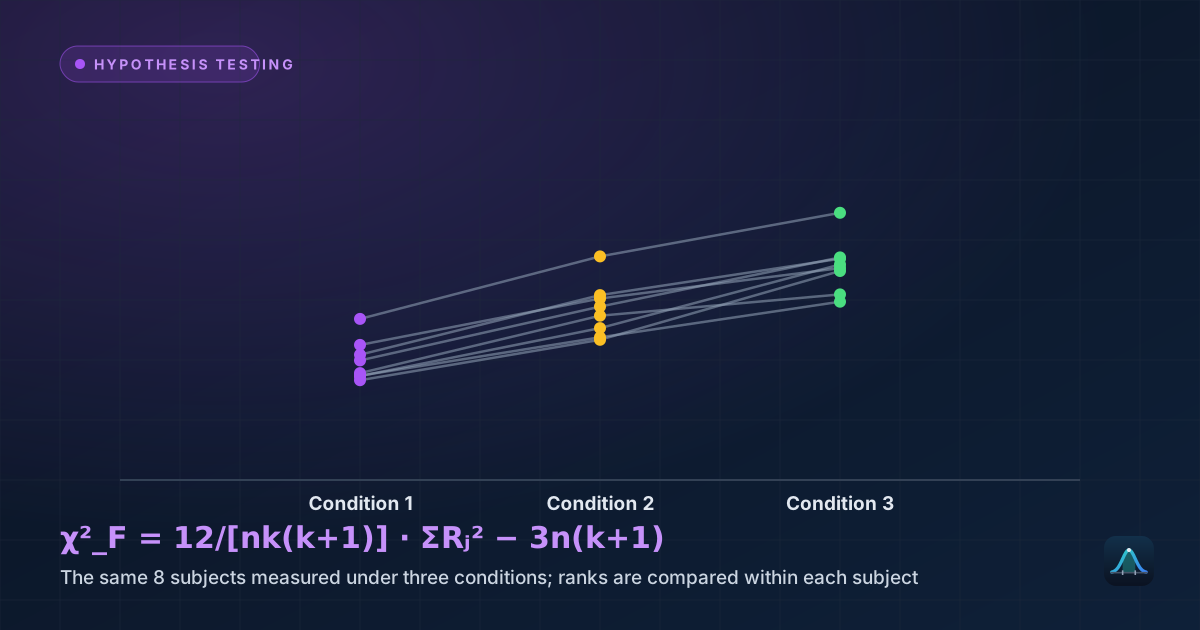
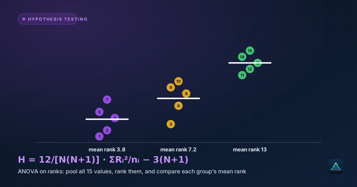
When ANOVA's normality assumption is seriously violated — heavily skewed data, small samples with visible non-normality, or ordinal (ranked) rather than genuinely continuous data — the Kruskal-Wallis test is the standard non-parametric alternative. It tests whether groups differ in their rank distributions rather than their means directly, trading some statistical power for a method that doesn't depend on a normality assumption. As with the choice between a t-test and its non-parametric counterparts, this is a real trade-off worth making deliberately, not a default to reach for automatically — ANOVA is more powerful when its assumptions genuinely hold.

What's the difference between one-way and two-way ANOVA?

One-way ANOVA tests the effect of a single categorical factor (like fertilizer type) on a continuous outcome. Two-way ANOVA tests the effect of two factors simultaneously (like fertilizer type AND soil type), and can also test whether the two factors interact — whether the effect of one depends on the level of the other.

Can ANOVA be used with just two groups?

Yes — with exactly two groups, one-way ANOVA and an independent two-sample t-test give mathematically equivalent results (F equals t², and the p-values match exactly). ANOVA's real advantage appears with three or more groups, where it correctly avoids the multiple-comparisons problem a series of t-tests would create.

What does it mean if F is close to 1?

An F close to 1 means between-group variance and within-group variance are roughly similar in size — consistent with the null hypothesis that all group means are actually equal, since there's no more variation between groups than you'd expect from ordinary random spread within each group.