Simple Linear Regression: The Least-Squares Line, Explained

Correlation tells you two variables move together. Regression goes a step further: it builds an actual equation that predicts one variable from the other. Simple linear regression fits a straight line through a set of data points — the same line that minimizes the total squared distance between the line and every point — turning a scatter of dots into a usable predictive model.

The Model

This builds directly on Pearson correlation: everywhere correlation measures how strongly two variables move together, regression takes the next step and turns that relationship into an equation you can actually use to make a prediction. Both share the same core limitation, worth restating here: neither proves causation on its own.

Here ŷ (read "y-hat") is the predicted value of y for a given x, b₀ is the y-intercept (the predicted y when x = 0), and b₁ is the slope (how much ŷ changes for each one-unit increase in x). The "hat" notation matters: ŷ is a prediction from the model, not the actual observed y — real data points almost never fall exactly on the line, and the vertical gap between each point and the line is called a residual.

Least Squares: How the Line Is Chosen

Of the infinite possible lines you could draw through a scatter of points, ordinary least squares (OLS) picks the one specific line that minimizes the sum of squared residuals — the total squared vertical distance between every point and the line. Squaring (rather than just summing raw distances) does the same job it does in variance: it makes every residual positive and penalizes larger errors disproportionately, so the method is especially sensitive to points that sit far from the general trend.

The slope and intercept that achieve this minimum have direct formulas:

Worked Example

Problem: An ice cream shop records daily temperature (°C) and ice creams sold: (18, 45), (22, 58), (25, 70), (28, 82), (30, 95). Fit a regression line and predict sales at 32°C.

x̄ = (18+22+25+28+30)/5 = 24.6. ȳ = (45+58+70+82+95)/5 = 70

Σ(xᵢ−x̄)(yᵢ−ȳ) = (−6.6)(−25)+(−2.6)(−12)+(0.4)(0)+(3.4)(12)+(5.4)(25) = 165+31.2+0+40.8+135 = 372

Σ(xᵢ−x̄)² = 43.56+6.76+0.16+11.56+29.16 = 91.2

Slope: b₁ = 372/91.2 ≈ 4.08

Intercept: b₀ = 70 − 4.08(24.6) ≈ 70 − 100.4 ≈ −30.4

Model: ŷ = −30.4 + 4.08x

Prediction at x = 32: ŷ = −30.4 + 4.08(32) = −30.4 + 130.6 = ≈ 100 ice creams

Interpretation of the slope: each 1°C increase in temperature is associated with about 4.08 more ice creams sold. The intercept (−30.4) is mathematically necessary to fit the line, but shouldn't be over-interpreted here — it predicts negative sales at 0°C, which is nonsensical; the model is only trustworthy within (or close to) the range of temperatures actually observed.

R²: How Well Does the Line Fit?

R² (the coefficient of determination) measures the proportion of variance in y that's explained by the linear relationship with x, ranging from 0 (the line explains none of the variation) to 1 (the line explains all of it). For simple linear regression, R² is simply the square of the Pearson correlation coefficient: R² = r². An R² of 0.85 means 85% of the variation in ice cream sales is associated with variation in temperature, leaving 15% explained by other factors (day of the week, local events, price changes, and so on) not captured in this simple model.

Residual Analysis: The Check R² Alone Won't Give You

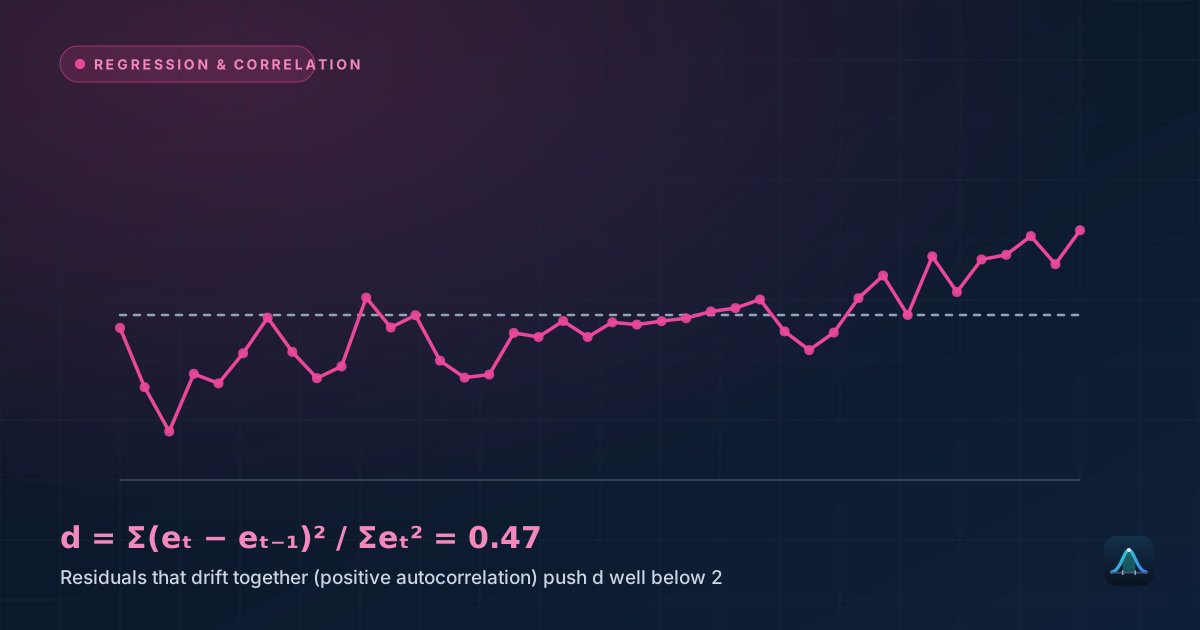
A residual plot — plotting each residual (actual y minus predicted ŷ) against x — is the standard diagnostic for whether a linear model is actually appropriate. Residuals scattered randomly around zero, with no visible pattern, support the linear model. A clear curve, funnel shape (widening or narrowing spread), or other systematic pattern in the residuals signals that a straight line is missing something real — perhaps the true relationship is curved, or the variability itself changes across the range of x (called heteroscedasticity), both of which violate assumptions the model relies on for its predictions and confidence intervals to be trustworthy.

Extrapolation: The Danger of Predicting Outside the Observed Range

The regression line was fit using temperatures between 18°C and 30°C. Using it to predict sales at 5°C or 45°C — well outside that range — is extrapolation, and it's genuinely risky: there's no data supporting the assumption that the same straight-line relationship continues to hold outside the observed range. Sales presumably don't keep climbing linearly forever as temperature rises, and likely don't go negative as it falls — the model's predictions become progressively less trustworthy the further you push beyond the data that built it.

Real-World Uses

Real estate valuation: regressing house price on square footage (or, more realistically, on many predictors simultaneously via multiple regression) is a standard technique behind automated home-value estimates, using historical sales data to fit a predictive model applied to new listings.

Economics: regression is the primary tool for estimating relationships like how consumer spending responds to income changes, or how demand for a product responds to price changes — quantifying relationships that pure theory can suggest the direction of, but not the precise magnitude.

Sports analytics: predicting player performance or game outcomes from measurable statistics (a well-known application: predicting baseball win totals from run differential) relies on regression to quantify exactly how strongly and in what direction each factor matters.

Scientific research: calibration curves — converting a measured instrument signal into a known physical quantity, like converting a spectrophotometer reading into a chemical concentration — are built using linear regression on known reference samples.

Common Mistakes

Fitting a straight line to an obviously curved relationship. Always look at the scatter plot before fitting a linear model — some relationships (population growth, radioactive decay, many biological processes) are fundamentally non-linear, and forcing a straight line through them, however high the resulting R², produces systematically biased predictions across parts of the range.

Letting a single influential outlier dominate the fit. Because least squares minimizes squared residuals, a single extreme point can pull the entire regression line toward itself far more than its "fair share" of influence would suggest. Checking for high-leverage points is a standard part of a careful regression analysis, not an optional extra step.

Reporting the slope without its uncertainty. A slope calculated from a small or noisy sample carries real uncertainty, just like any other sample statistic — reporting a confidence interval or standard error for the slope, not just its point estimate, gives a much more honest picture of how precisely the relationship has actually been pinned down.

Simple vs. Multiple Regression

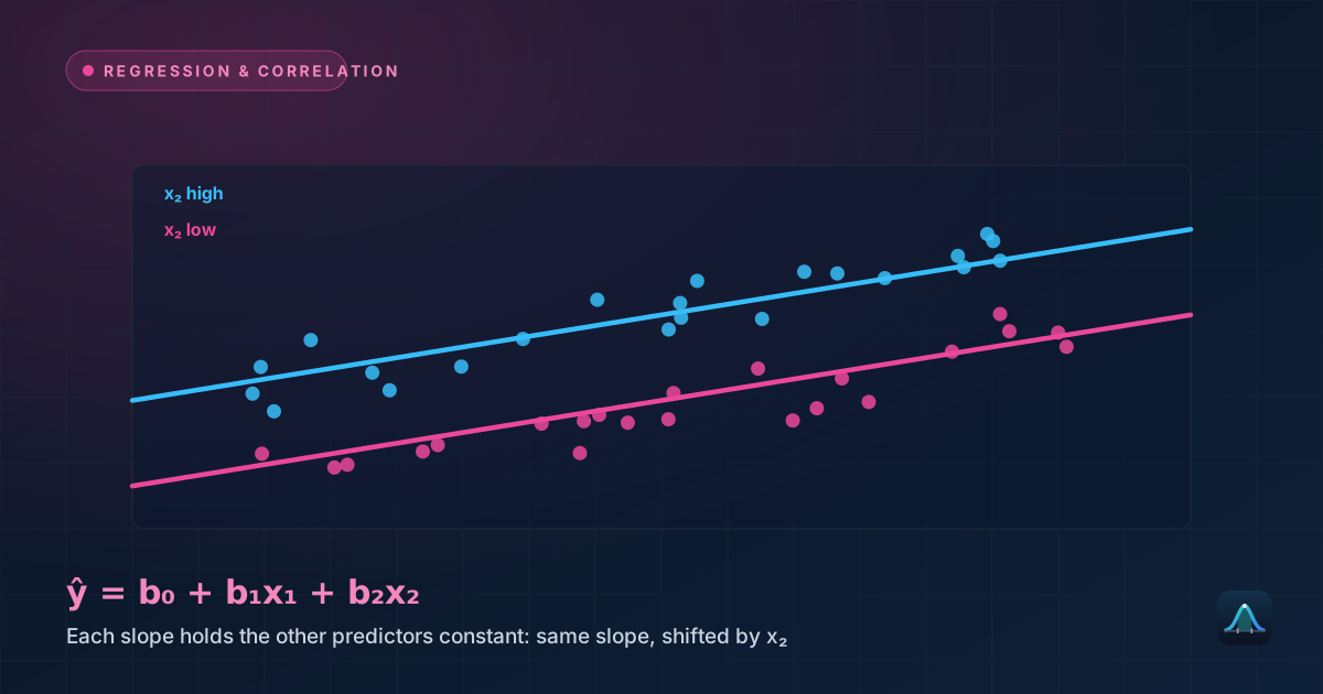
Simple linear regression uses exactly one predictor variable. Multiple regression extends the same underlying idea to several predictors simultaneously (ŷ = b₀ + b₁x₁ + b₂x₂ + ...), letting a model account for several factors at once — predicting ice cream sales from temperature AND day-of-week AND local event calendar, for instance, typically explaining more of the variation than temperature alone and untangling each predictor's individual contribution.