The Durbin-Watson Test: Detecting Autocorrelation in Regression Residuals

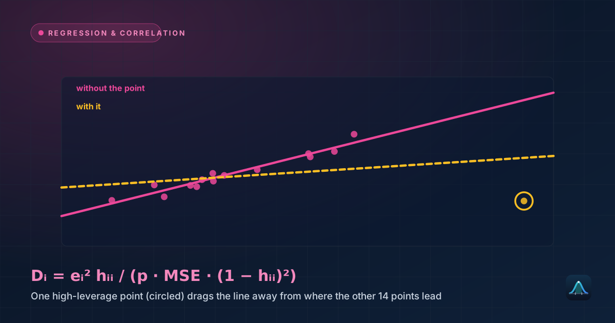
Linear regression assumes each observation's error is independent of the others. When your data is a time series, that assumption often breaks: a residual that's too high this month tends to stay too high next month, because whatever the model is missing (a trend, a season, a slow-moving factor) doesn't reset every period. The Durbin-Watson test checks for exactly this — first-order autocorrelation in regression residuals — and is one of the standard diagnostics run alongside any regression fit to time-ordered data — a natural companion to checking influential points and residual normality before trusting a model's p-values.

The Statistic

where e₁, ..., eₙ are the regression residuals in time order. When consecutive residuals tend to be close to each other (positive autocorrelation), the differences in the numerator are small, so d is small — down toward 0. When residuals swing back and forth from one period to the next (negative autocorrelation), the differences are large, pushing d up toward 4. With no autocorrelation, d lands near 2.

Why Bounds Instead of a Single Critical Value

Most test statistics on this site have a critical value that depends only on the sample size (and maybe the number of groups or parameters). The Durbin-Watson statistic is different: its exact null distribution depends on the actual values of the regressors X, which differ from dataset to dataset. Durbin and Watson's key result was that regardless of what X actually is, the true critical value always falls between two bounds — dL and dU — that depend only on n and the number of parameters. That gives a valid, if occasionally inconclusive, test: d below dL always rejects the null of no autocorrelation, d above dU never does, and dL ≤ d ≤ dU means the test can't say either way without more information (some software computes an exact p-value for the specific X instead, sidestepping the gap — the bounds remain the standard hand-calculation approach).

Worked Example: A Missed Seasonal Pattern

Problem: A regression forecasts monthly sales from a single predictor (marketing spend) across 15 months, but the residuals, in order, are: −3, −2, −1, 0, 1, 2, 3, 2, 1, 0, −1, −2, −3, −2, −1. Is there autocorrelation?

The pattern is visible immediately — the residuals rise smoothly, peak, and fall smoothly, like a wave, rather than jumping around at random. Computing d directly: the sum of squared consecutive differences Σ(eₜ−eₜ₋₁)² = 14, and the sum of squared residuals Σeₜ² = 52, so d = 14/52 ≈ 0.269.

With n=15 and k=1 predictor (so 2 parameters including the intercept), the exact bounds at α=0.05 are dL=1.077 and dU=1.361. The observed d=0.269 is far below dL, so the test rejects the null hypothesis of no autocorrelation — strong evidence of positive autocorrelation. In practice, this residual pattern (a smooth rise and fall) is exactly what you'd see if the model were missing a seasonal component that a plain trend line can't capture.

What to Do About Autocorrelated Residuals

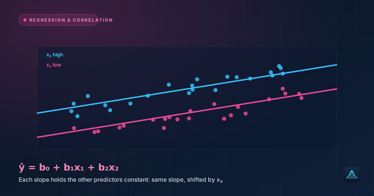
A significant Durbin-Watson result doesn't mean the regression is wrong to run — it means the standard errors and p-values from ordinary least squares are no longer trustworthy, because they assume independent errors. Common fixes include adding the missing structure directly — a trend term, seasonal dummy variables, or a lagged version of the outcome as a predictor — or, if the predictors involve more than one variable, revisiting the multiple regression specification itself. Some analysts instead use an estimation method built for autocorrelated errors (such as Newey-West standard errors), which corrects the standard errors without changing the coefficients themselves. The same residual pattern that trips the Durbin-Watson test is also what the trend and seasonality decomposition covered elsewhere on this site is designed to separate out in the first place.

Common Mistakes

Using it on non-time-series data. The test is specifically about order — it assumes the data has a natural sequence (usually time). Running it on cross-sectional data with an arbitrary row order produces a meaningless result, since "consecutive" rows aren't meaningfully connected.

Ignoring the inconclusive zone. When d falls between dL and dU, the honest conclusion is "the bounds test can't say" — treating it as a pass (like d above dU) overstates how much the diagnostic actually cleared.

Forgetting it only catches first-order autocorrelation. The test is built to detect correlation between a residual and the one immediately before it. More complex patterns — correlation with a residual several periods back, or seasonal cycles — can slip past a Durbin-Watson test that looks perfectly fine, which is why a residual plot is still worth checking directly.