Polynomial Regression: Fitting a Curve Instead of a Straight Line

Simple linear regression fits the single best straight line through a scatter of points — but not every real relationship is a straight line. When a relationship genuinely curves (rises, then falls; accelerates, then levels off), polynomial regression extends the same least-squares idea to fit a curve instead, by adding powers of x (x², x³, and so on) as additional predictors.

The Model

A quadratic (degree-2) polynomial regression model takes the form:

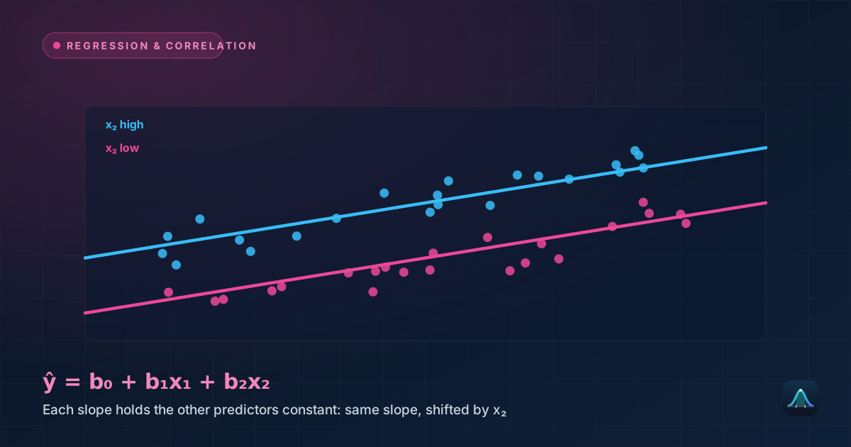
This might look like a fundamentally different technique from simple linear regression, but it's actually a direct extension of the same multiple linear regression machinery: x² is simply treated as a second predictor variable, computed directly from x. The model is still "linear" in the technical statistical sense — linear in its coefficients (b₀, b₁, b₂), even though the resulting curve plotted against x is not a straight line at all. This is why the same least-squares fitting method, and the same R² interpretation, carry over directly from ordinary linear regression.

Worked Example: Study Hours and Test Performance

Problem: A researcher records hours studied and test scores for 7 students: (1, 52), (2, 68), (3, 78), (4, 85), (5, 88), (6, 86), (7, 80). Scores clearly rise with more study time — but then start falling after about 5 hours, presumably reflecting fatigue or diminishing returns. Compare a linear fit to a quadratic fit.

A plain linear regression on this data gives ŷ = 58.14 + 4.64x, with R² ≈ 0.615 — a fit that misses the pattern badly, since a straight line can't capture the rise-then-fall shape and is forced to average across it.

Fitting a quadratic model to the same data (using the same least-squares principle, extended to solve for three coefficients instead of two) gives:

with R² ≈ 0.999 — an almost perfect fit, dramatically better than the linear model's 0.615. The negative coefficient on x² (−2.12) is what produces the downward curve: as x grows large enough, the x² term's negative contribution eventually outweighs the positive linear term, pulling predicted scores back down — exactly the fatigue effect visible in the raw data.

Finding the Turning Point

For a quadratic ŷ = b₀ + b₁x + b₂x², the curve's peak (or trough, if b₂ is positive) occurs at:

For the worked example: x = −21.60 / (2 × −2.12) ≈ 5.10. The model predicts peak performance at around 5.1 hours of studying, with a predicted score of approximately 87.7 at that point — closely matching the actual peak visible in the raw data (88 points, at x=5), and giving a concrete, actionable number ("around 5 hours") that a straight-line model couldn't have produced at all.

The Overfitting Risk

Adding more polynomial terms (x³, x⁴, and beyond) always increases R² — a higher-degree polynomial has more flexibility to bend and twist through the data points, and with enough terms, a curve can be made to pass through every single data point exactly, driving R² all the way to 1. This is not a genuine improvement: a curve contorted to hit every point exactly is almost always overfit — it's capturing random noise specific to this dataset rather than the real underlying pattern, and it will typically make poor predictions on new data it wasn't fit to, in the same overfitting sense that shows up in machine learning's bias-variance tradeoff. A rising R² alone is never sufficient justification for adding another polynomial term — the added complexity needs to be justified by genuinely improved out-of-sample prediction, not just a better fit to the exact data already in hand.

Choosing the Right Degree

Start by looking at the scatter plot. A single clear bend (one rise, one fall, or vice versa) suggests a quadratic (degree-2) term might help; a more complex wiggling pattern with multiple direction changes would need a higher degree, but also raises the overfitting concern discussed above much sooner.

Check whether the higher-degree term is actually justified statistically, not just by eyeballing R² — a significance test on the x² coefficient itself (is it significantly different from zero?) is the more rigorous way to decide whether the added curve genuinely improves the model or is just fitting noise.

Be especially cautious extrapolating beyond the observed x-range. Polynomial curves can behave wildly just outside the range of the data used to fit them — a quadratic that looks like a gentle, sensible curve within the observed range can shoot off toward implausible predictions almost immediately beyond it, an even sharper version of the extrapolation danger already flagged for ordinary linear regression.

Real-World Uses

Dose-response and yield curves: many biological and agricultural relationships genuinely rise then plateau or decline (crop yield versus fertilizer amount, drug effect versus dosage), making quadratic or low-degree polynomial models a natural and commonly used fit.

Physical motion and trajectories: a projectile's height over time famously follows a quadratic curve, and polynomial regression is a standard way to fit real, noisy trajectory data back to the underlying physical model when the exact physical parameters aren't known in advance.

Economic cost and revenue curves: production costs or revenue often follow curved, rather than strictly linear, relationships with quantity produced or sold, reflecting effects like economies of scale at low volumes and diminishing returns at high volumes — both captured naturally by a polynomial term where a straight line would systematically misrepresent one end of the range or the other.

Common Mistakes

Adding polynomial terms just because R² improves. As explained above, R² always rises (or at worst stays the same) with each added term — this alone is never sufficient justification, since it happens even when the added term is fitting pure noise.

Extrapolating a polynomial fit beyond the observed data range. This is a much sharper version of the risk already present in simple linear regression, since polynomial curves can swing dramatically once pushed outside the range of x-values they were actually fit to.

Forgetting that a quadratic model implies a symmetric curve around its turning point. Real relationships aren't always symmetric — a quadratic model forces symmetry around its peak or trough whether or not the real underlying pattern actually behaves that way, which is worth checking against the raw data visually.