The Uniform Distribution: Formula, Worked Examples, and When to Use It

Most of the distributions covered elsewhere on this site — the normal distribution, the binomial distribution — describe outcomes that cluster around some central, most-likely value. The uniform distribution describes the opposite situation: every outcome in a range is equally likely, with no peak, no cluster, and no tendency toward any particular value at all. A bus that could arrive at any minute within a 20-minute window, a random number generator producing any decimal between 0 and 1, a spinner landing on any angle around a circle — all follow a uniform distribution.

Continuous vs. Discrete Uniform

The uniform distribution comes in two versions, and it matters which one a problem describes. The discrete uniform distribution applies to a finite, countable set of equally likely outcomes — rolling a fair die (six outcomes, each with probability 1/6) is the textbook example. The continuous uniform distribution applies when the outcome can be any real number within an interval [a, b], not just whole numbers — a bus arriving anywhere within a 20-minute window is continuous, because the arrival time isn't restricted to whole minutes. This guide focuses mainly on the continuous case, since it's the one that shows up most often in applied statistics and connects most directly to other distributions on this site.

The Continuous Uniform Distribution

For a continuous uniform distribution over the interval [a, b], every sub-interval of the same width has the same probability, regardless of where it falls within [a, b]. The probability density function is constant across the whole interval and zero everywhere else:

This constant height is exactly what makes the distribution's graph a flat rectangle rather than a curve — the defining visual signature of "uniform." Because the total area under any probability density function must equal 1, and the rectangle's width is (b−a), its height must be 1/(b−a) for the area to work out to exactly 1.

Finding the probability that X falls between two values c and d (where a ≤ c ≤ d ≤ b) is simple precisely because the density is constant — it's just the proportion of the total range that [c, d] covers:

Mean and Standard Deviation

By symmetry, the mean of a uniform distribution always falls exactly halfway between a and b:

The standard deviation formula looks less intuitive than the mean, but it follows directly from integrating the squared distance from the mean across a flat density — the constant √12 in the denominator comes out of that calculus and is worth simply memorizing rather than re-deriving each time.

Worked Example: Bus Wait Time

Problem: A bus arrives at a stop at a uniformly random time between 0 and 20 minutes after you get there. What's the probability you wait between 5 and 15 minutes? What are the mean and standard deviation of your wait time?

Here a = 0 and b = 20, so the density height is f(x) = 1/(20−0) = 0.05 for any wait time between 0 and 20 minutes.

P(5 ≤ X ≤ 15) = (15−5) / (20−0) = 10/20 = 0.5

There's exactly a 50% chance of waiting between 5 and 15 minutes — which makes sense, since that 10-minute window is exactly half of the full 20-minute range, and every equal-width window carries equal probability under a uniform distribution.

μ = (0+20)/2 = 10 minutes, and σ = (20−0)/√12 ≈ 20/3.464 ≈ 5.77 minutes. On average you'll wait 10 minutes, with wait times typically varying by around 5.77 minutes from that average.

Worked Example: Ride-Share Pickup

Problem: A ride-share app quotes pickup times as uniformly distributed between 2 and 12 minutes. What's the probability the driver takes more than 9 minutes? What's the expected pickup time?

Here a = 2 and b = 12, so the total range is 10 minutes. The event "more than 9 minutes" covers the sub-interval from 9 to 12, a width of 3 minutes.

P(X > 9) = (12−9) / (12−2) = 3/10 = 0.3

There's a 30% chance of waiting more than 9 minutes for pickup. The expected pickup time is μ = (2+12)/2 = 7 minutes, with a standard deviation of σ = (12−2)/√12 ≈ 2.89 minutes.

The Discrete Uniform Distribution

When outcomes are countable rather than continuous — rolling a fair die, picking a random integer from 1 to n, drawing a raffle ticket number — the discrete uniform distribution applies instead. For n equally likely outcomes, each has probability exactly 1/n, and the formulas for mean and variance take a similar but distinct form:

For a fair six-sided die (n=6): each face has probability 1/6, the mean outcome is (6+1)/2 = 3.5 (which is why 3.5 is often quoted as "the average die roll," even though 3.5 can never actually be rolled), and the variance is (36−1)/12 ≈ 2.92.

Why the Uniform Distribution Matters Beyond These Examples

Random number generation: nearly every computer's random number generator is built on producing values from a continuous uniform distribution on [0, 1] as its foundation — every other distribution used in simulation (normal, binomial, exponential, and the rest) is generated by mathematically transforming uniform random values, making the uniform distribution the quiet building block underneath almost all randomness in software.

A neutral prior in Bayesian statistics: when there's genuinely no reason to favor one value over another before seeing any data, a uniform distribution is the natural choice to represent that lack of prior information — see the discussion of priors in Bayesian vs. frequentist statistics.

Rounding error: when a continuous measurement is rounded to the nearest unit, the rounding error itself is well-modeled as uniformly distributed between −0.5 and +0.5 of that unit — a common assumption in measurement-error analysis.

Benchmark for "no pattern": testing whether observed data is uniformly distributed (using a chi-square goodness-of-fit test) is a standard way to check for genuine randomness — a slot machine's outcomes, a hash function's output distribution, or a lottery's drawn numbers should all look uniform if the underlying process is fair.

Uniform vs. Normal: Why the Shape Matters

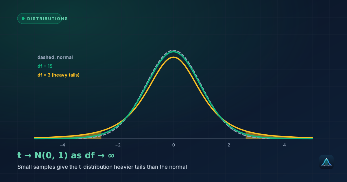
It's worth being explicit about the contrast with the normal distribution, since the two get confused. The normal distribution concentrates probability near its mean and tapers off toward the extremes — most outcomes land close to average, and far-from-average outcomes are rare. The uniform distribution has no such concentration: every value in its range is exactly as likely as every other, including the extremes. A striking connection ties them together despite this difference: if you take the average of many independent uniform random variables, that average becomes approximately normally distributed as the number of variables grows — a direct consequence of the Central Limit Theorem, and a reminder that the CLT applies regardless of how unusual the original distribution's shape is.

Common Mistakes

Treating a bell-shaped or skewed dataset as uniform. Real-world data is uniform far less often than it's normal, skewed, or otherwise shaped — confirm the assumption (a histogram is usually enough) before applying uniform-distribution formulas, rather than defaulting to "uniform" just because a range of possible values is known.

Confusing the continuous and discrete formulas. The variance formulas differ ((b−a)²/12 for continuous, (n²−1)/12 for discrete) because they're built on genuinely different underlying models — mixing them up gives a wrong answer even though the results look superficially similar.

Assuming probability equals width without dividing by the total range. P(c ≤ X ≤ d) is the proportion of the total range covered by [c, d], not just the raw width (d−c) — forgetting to divide by (b−a) is a common arithmetic slip, especially when a and b aren't 0 and 1.

Can the uniform distribution have a negative range?

Yes — a and b just need a < b; the interval can span negative numbers, cross zero, or lie entirely below zero (for example, a temperature error uniformly distributed between −2°C and +2°C). Only the width (b−a) matters for the formulas, not where the interval sits on the number line.

What does the cumulative distribution function look like?

Because the density is constant, the cumulative distribution function is a straight line rising steadily from 0 at x=a to 1 at x=b, given by F(x) = (x−a)/(b−a) — a direct consequence of probability accumulating at a constant rate across a flat density.

Is the standard uniform distribution the same as "uniform"?

"Standard uniform" specifically means the continuous uniform distribution on [0, 1] — the special case with a=0 and b=1. It's called out separately because it's the default building block most software's random number generators actually produce, with every other interval or distribution derived from it.

Why is the variance formula (b−a)²/12 and not something simpler?

The 12 comes from formally integrating (x−μ)² times the constant density 1/(b−a) across the interval [a,b] — the calculus works out cleanly to (b−a)²/12. It's not an arbitrary constant; it's simply the value that specific integral evaluates to, and it's standard to treat it as a fixed formula rather than re-deriving it each time.