The Central Limit Theorem, Explained With Worked Examples

The Central Limit Theorem is the single result that makes most of modern statistics possible. It's also one of the most counterintuitive: it makes a strong, precise claim about the shape of a distribution that holds true almost regardless of what the underlying data actually looks like. Once you understand why it works, an enormous amount of statistical machinery — confidence intervals, hypothesis tests, quality control charts — stops looking like a grab-bag of separate techniques and starts looking like one idea applied repeatedly.

The Claim, Precisely Stated

Take repeated random samples of size n from any population, no matter its shape — skewed, bimodal, uniform, wildly irregular. Calculate the mean of each sample. The Central Limit Theorem (CLT) states that as n grows large, the distribution of those sample means approaches a normal distribution, centred on the true population mean, regardless of the shape of the original population.

Read that carefully: it's not saying your data becomes normally distributed. Your original data can stay exactly as skewed or strange as it always was. It's the distribution of sample means — a completely different thing — that becomes approximately normal.

Why This Is Surprising

Imagine a population of customer wait times that's heavily right-skewed: most customers wait a short time, but a long tail occasionally waits much longer. If you take a single sample of 30 customers and average their wait times, that one average could land almost anywhere. But if you repeated this — took a fresh sample of 30, averaged it, took another fresh sample of 30, averaged that too, and did this thousands of times — the resulting collection of thousands of averages would pile up into a bell-shaped, normal distribution, centred right on the true population mean. The skew in the original data essentially washes out through the act of averaging.

This happens because averaging is a smoothing operation. Any single extreme value in a sample gets diluted by the other n−1 values around it. Extreme sample means (way too high or way too low) require an unusual run of extreme individual values all landing in the same sample — which becomes rapidly less likely as the sample size grows, and the mathematics of that "rapidly less likely" shape turns out to converge on the normal curve specifically, regardless of the original population's shape.

How Large Does n Need to Be?

The rule of thumb taught in most introductory courses is n ≥ 30. This is a genuinely useful default, but it's a rule of thumb, not a hard law written into the mathematics. The real answer is "it depends on how far from normal the original population already is":

• If the population is already roughly symmetric and unimodal, the sampling distribution of the mean looks close to normal even for quite small samples (n = 10 or less).
• If the population is heavily skewed or has extreme outliers, you may need a considerably larger sample — sometimes well beyond 30 — before the sampling distribution looks convincingly normal.
• n = 30 is a reasonable, conservative default for moderately-shaped real-world data, which is exactly why it became the standard teaching heuristic — not because 30 is mathematically special.

Standard Error: How Spread Out Are the Sample Means?

The CLT tells you the sampling distribution of the mean is approximately normal, but it also tells you exactly how spread out that distribution is — this spread is called the standard error:

Notice the √n in the denominator: as sample size grows, standard error shrinks — but not proportionally. Quadrupling your sample size only halves the standard error, because of the square root. This is the mathematical reason why survey sample sizes have famously diminishing returns: going from 100 to 1,000 respondents tightens your estimate a lot; going from 1,000 to 10,000 tightens it much less, for ten times the cost and effort.

Worked Example

Problem: A factory's bolt lengths have a population mean of 50mm and a population standard deviation of 4mm (the underlying distribution of individual bolt lengths is unknown and possibly skewed). If you take random samples of n = 64 bolts and calculate each sample's mean length, what is the standard error of those sample means, and within what range would you expect 95% of sample means to fall?

Standard error: SE = σ/√n = 4/√64 = 4/8 = 0.5mm

95% range (using the empirical rule, ±2 SE): 50 ± 2(0.5) = 50 ± 1 = 49mm to 51mm

Even though we know nothing about the shape of individual bolt lengths, the CLT guarantees that with n = 64, the distribution of sample means is close enough to normal that this ±2 SE range genuinely captures about 95% of possible sample means — this is the exact mechanism that makes confidence intervals mathematically valid.

What the CLT Does Not Say

It's worth being precise about the theorem's limits, since these are exactly where students go wrong:

• It does not claim your raw data becomes normal — only the distribution of sample means (or sums, or several other summary statistics) does.
• It does not work for very small samples from heavily skewed populations — the approximation genuinely can be poor at, say, n = 5 from a strongly skewed source.
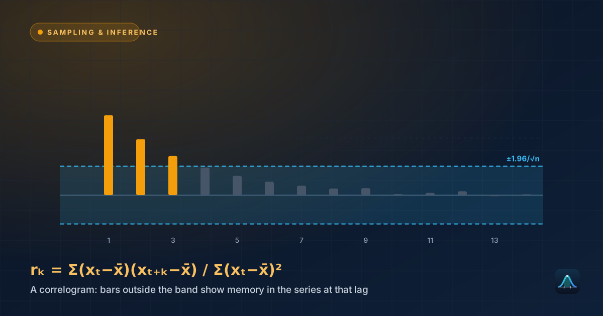
• It requires samples to be independent and identically distributed (drawn randomly, without one observation influencing another) — the theorem breaks down for data with strong internal correlation, such as many time series.

Simulating It Yourself

The fastest way to build real intuition for the CLT is to watch it happen. Take any wildly non-normal distribution — even something as extreme as a uniform distribution, or dice rolls (which have a flat, rectangular distribution, not a bell curve at all). Roll one die repeatedly and plot the individual outcomes: you'll get a flat distribution, each face equally likely. Now roll five dice at a time, take the average of each group of five, and plot those averages instead: the result visibly humps into a rough bell shape, even from a source distribution that has no bell shape whatsoever. This is the CLT operating in the simplest possible case, and it's a genuinely useful classroom demonstration for exactly this reason.

Where the CLT Shows Up in Practice

Quality control charts: manufacturers plot the mean of small samples of parts (not individual parts) over time precisely because the CLT guarantees those sample means will be approximately normally distributed, letting engineers use fixed, mathematically justified control limits (commonly ±3 standard errors) to flag a process drifting out of spec.

Political polling: a poll of 1,000 randomly selected voters produces a sample proportion. The CLT (in its proportion form) is what justifies reporting a margin of error like "±3 percentage points" — a number that would be meaningless to calculate without the theorem guaranteeing the sampling distribution's shape.

A/B testing: when a company compares conversion rates between two versions of a webpage, the statistical test behind the "is this difference significant?" decision relies on the CLT to justify treating the difference between two sample means as approximately normally distributed, even though individual visitor behaviour (converted or didn't) is about as far from normal as data gets — it's binary.