The normal distribution — the familiar bell-shaped curve — is the single most important distribution in statistics, not because nature has some special preference for bells, but because it emerges naturally whenever many small, independent factors add together to produce an outcome. Human height, measurement error, blood pressure, and standardized test scores all approximate it closely, and even when the underlying data doesn't, the Central Limit Theorem guarantees that sample means drawn from almost any distribution will.
- What makes the normal distribution's shape special, mathematically
- The 68-95-99.7 empirical rule and how to actually use it
- How to find probabilities for any range using z-scores
- When real data does — and doesn't — genuinely follow a normal distribution
The Shape, and What Defines It
A normal distribution is fully described by exactly two numbers: its mean (μ), which sets the centre and peak of the curve, and its standard deviation (σ), which sets how wide or narrow the curve is. The curve is perfectly symmetric around the mean, single-peaked, and its tails extend infinitely in both directions without ever quite touching zero — though the probability out in the far tails becomes vanishingly small.
You'll rarely need to use this formula directly — in practice, probabilities are found using a z-table, software, or a calculator — but it's worth seeing once: notice the (x−μ)² term, which is exactly why the curve is symmetric (squaring removes the sign, so equal distances above and below the mean produce equal heights).
The 68-95-99.7 Empirical Rule
For any normal distribution, the proportion of data within a fixed number of standard deviations of the mean is always the same:
- About 68% of values fall within 1 standard deviation of the mean (μ ± σ)
- About 95% of values fall within 2 standard deviations (μ ± 2σ)
- About 99.7% of values fall within 3 standard deviations (μ ± 3σ)
This is one of the most useful facts in applied statistics because it gives you an immediate, no-calculation sense of "how unusual" a value is, just from knowing the mean and SD. A value more than 2 SD from the mean is already in roughly the most extreme 5% of the distribution; beyond 3 SD, it's in the most extreme 0.3% — genuinely rare.
Worked Example: Applying the Empirical Rule
Problem: Adult resting heart rate is approximately normally distributed with mean μ = 70 bpm and standard deviation σ = 8 bpm. What range covers approximately 95% of adults, and what proportion have a resting heart rate above 86 bpm?
95% range: μ ± 2σ = 70 ± 16 = 54 bpm to 86 bpm
Above 86 bpm: 86 is exactly 2 SD above the mean. Since 95% falls within ±2σ, the remaining 5% is split evenly between the two tails (by symmetry) → 2.5% falls above 86 bpm, and 2.5% falls below 54 bpm.
Beyond the Empirical Rule: Any Probability, Using Z-Scores
The empirical rule only covers exact multiples of 1, 2, and 3 standard deviations. For any other value, convert to a z-score — z = (x−μ)/σ — and look up the corresponding probability in a standard normal table, or use software. This works because every normal distribution, once converted to z-scores, maps onto the exact same standard normal curve (mean 0, SD 1), which has been precisely tabulated.
Example: what proportion of the resting-heart-rate population above falls below 78 bpm? z = (78−70)/8 = 1.0. A standard normal table gives P(Z < 1.0) ≈ 0.8413 — so about 84.1% of adults have a resting heart rate below 78 bpm.
Does Real Data Actually Follow a Normal Distribution?
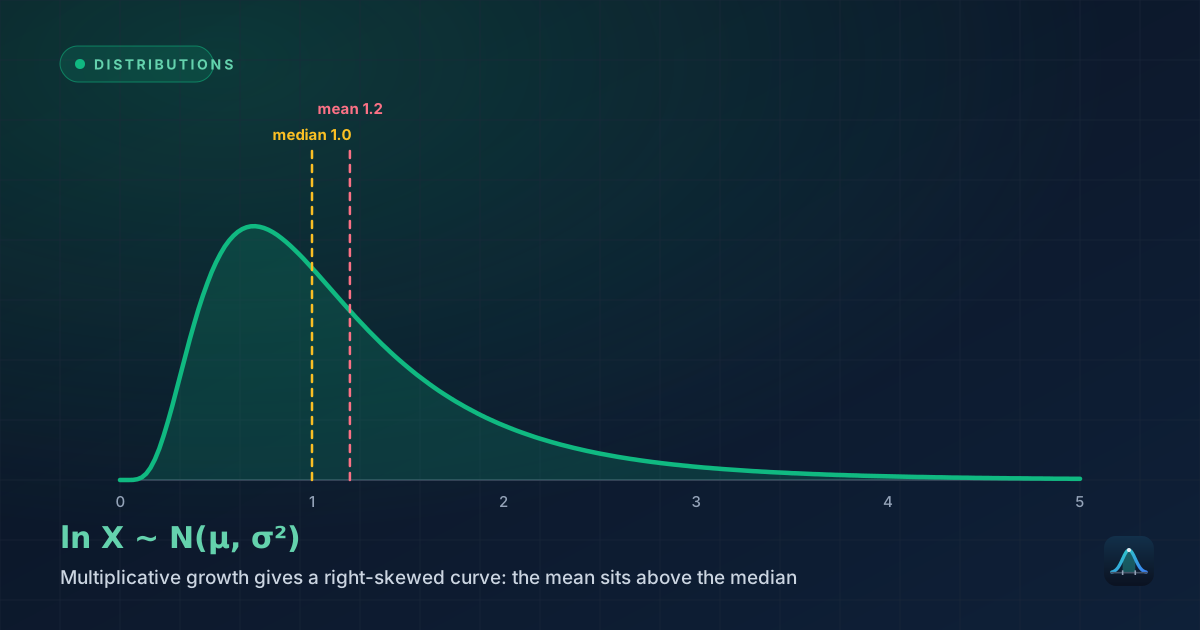
Often approximately, but rarely exactly, and it's worth being honest about the difference. Many biological and physical measurements (height, blood pressure, measurement error) are close enough to normal that the approximation works well for practical purposes. But plenty of common real-world data is genuinely non-normal: income and house prices are right-skewed; the number of customers arriving per hour often follows a Poisson distribution instead; reaction times typically have a long right tail. Formal normality tests (like the Shapiro-Wilk test) exist precisely because "does this look bell-shaped" isn't always obvious from a histogram alone, and many statistical methods (like t-tests) rely on a normality assumption that should genuinely be checked, not assumed.
The Central Limit Theorem is the deeper reason the normal distribution is everywhere in statistical practice, even when individual data points aren't normally distributed. Averages and sums of many independent random contributions tend toward a normal shape regardless of the shape of each individual contribution — this is why sampling distributions of the mean are usually treated as approximately normal, even when the underlying population clearly isn't.
Standard Deviation and the Shape of the Curve
Two normal distributions can have the same mean but look very different depending on their standard deviation. A small σ produces a tall, narrow curve — values cluster tightly around the mean. A large σ produces a short, wide curve — values are spread out considerably. This is why standard deviation, not just the mean, is essential to fully describe a normal distribution: knowing only "the average is 70" tells you nothing about whether most values are close to 70 or scattered widely around it.
Applications
Manufacturing tolerances: component dimensions are often modelled as normally distributed around a target value, with the empirical rule used to set realistic tolerance bands and estimate defect rates.
Standardized testing: raw scores are frequently transformed to follow a normal distribution with a fixed mean and SD (like IQ tests, standardized at mean 100, SD 15), making results comparable across different test versions and years.
Natural and social sciences: traits shaped by many small, additive genetic and environmental factors — adult height, blood pressure, IQ scores by construction — tend to follow the normal distribution closely, which is part of why the curve was historically first studied in this context (originally called the "Gaussian" distribution, after Carl Friedrich Gauss's work on measurement error in astronomy).
Finance: stock returns are often modelled as approximately normal over short time horizons — a simplification that's useful but famously breaks down during extreme market events, where real returns show far "fatter tails" than a true normal distribution would predict.
What If the Data Isn't Normal? Chebyshev's Inequality
The 68-95-99.7 rule only holds for genuinely normal (or close to normal) data. For data of unknown or non-normal shape, a weaker but universally valid guarantee exists: Chebyshev's inequality, which states that for ANY distribution, at least (1 − 1/k²) of values fall within k standard deviations of the mean. For k = 2, that's at least 75% (compared to the normal distribution's 95%) — a much looser bound, but one that requires no assumption about shape at all. This is a useful fallback whenever you can't be confident your data is approximately normal but still want some guaranteed statement about how spread out it is.
A Second Worked Example
Problem: A machine fills cereal boxes with a mean weight of 500g and standard deviation of 5g, and the fill weight is approximately normally distributed. Quality control rejects any box below 490g. What percentage of boxes get rejected?
Z-score for 490g: z = (490 − 500) / 5 = −10/5 = −2.0
Interpretation: 490g is exactly 2 standard deviations below the mean. By the empirical rule, 95% of boxes fall within ±2σ (between 490g and 510g), leaving 5% outside that range, split evenly by symmetry — so approximately 2.5% of boxes fall below 490g and get rejected.
This kind of calculation is exactly what quality engineers use to set tolerance limits that balance an acceptable rejection rate against the cost of tightening the manufacturing process itself — tightening σ (making the machine more precise) is usually the real lever available, since shifting μ or the cutoff alone just trades one problem for another.
What's the difference between a normal distribution and the standard normal distribution?
Can a normal distribution produce negative values?
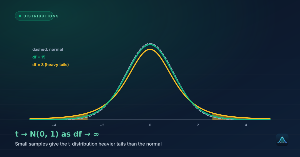
How is the normal distribution different from the t-distribution?
Why is 99.7% used as the "almost everything" threshold, not 100%?
Share this article
Written by
Statistics Fundamentals Editorial Team
Written and reviewed by our team of statistics educators. Content is aligned with GCSE, A-Level, AP Statistics, and undergraduate curricula.
About Statistics Fundamentals →