Partial Correlation: Controlling for a Third Variable

Pearson correlation measures how two variables move together — but that raw relationship can be inflated, or even entirely created, by both variables independently being related to some third factor. Partial correlation strips out that shared influence, revealing what the relationship between two variables actually looks like once a third variable's effect has been mathematically removed from both. It's one of the most direct, hands-on ways to see confounding in action, using nothing more than three ordinary correlation coefficients already familiar from elsewhere on this site.

The Formula

Given three variables X, Y, and Z, the partial correlation between X and Y, controlling for Z, is calculated from the three ordinary pairwise Pearson correlations among all three variables:

The notation r_XY.Z is read "the correlation between X and Y, controlling for Z." The numerator subtracts out the portion of the X-Y correlation that's mathematically attributable to both variables' shared relationship with Z; the denominator rescales the result back into the familiar −1-to-+1 range. Notice that all three inputs are ordinary Pearson correlations, already covered elsewhere on this site — computing a partial correlation doesn't require any new raw-data formula, just this one additional adjustment step applied to correlations already in hand.

Worked Example: Ice Cream Sales and Drowning Incidents

Problem: Across a series of summer months, ice cream sales and drowning incidents show a strong positive correlation, r_XY = 0.70. Both variables are also strongly related to temperature: ice cream sales and temperature correlate at r_XZ = 0.90, and drownings and temperature correlate at r_YZ = 0.80. What's the partial correlation between ice cream sales and drownings, controlling for temperature?

r_XY.Z = (0.70 − 0.90×0.80) / √[(1−0.90²)(1−0.80²)] = (0.70 − 0.72) / √[(0.19)(0.36)] = −0.02 / √0.0684 ≈ −0.076

Once temperature's shared influence is removed, the partial correlation between ice cream sales and drownings collapses from a seemingly strong 0.70 down to essentially zero (−0.076). The original correlation wasn't describing a real relationship between ice cream and drowning at all — both simply rise together on hot days, for entirely separate reasons (more people buy ice cream in the heat; more people also swim, and therefore face more drowning risk, in the heat). Temperature was the hidden variable doing all the real work, exactly the kind of confounding relationship covered in Pearson correlation's discussion of why correlation doesn't imply causation. No amount of staring harder at the raw ice-cream-versus-drowning scatter plot would reveal this — the confound only becomes visible once temperature is explicitly brought into the calculation.

A Second Worked Example: When Controlling Reveals a Stronger Relationship

Problem: A researcher studies hours studied (X) and exam score (Y), finding r_XY = 0.6. Both variables also relate to a student's anxiety level (Z): hours studied and anxiety correlate at r_XZ = 0.5, and exam score and anxiety correlate at r_YZ = 0.7 — anxious students tend to study more (perhaps out of worry) but anxiety itself tends to hurt exam performance, partially masking how effective the studying actually is. What's the partial correlation between hours studied and exam score, controlling for anxiety?

r_XY.Z = (0.6 − 0.5×0.7) / √[(1−0.5²)(1−0.7²)] = (0.6 − 0.35) / √[(0.75)(0.51)] = 0.25 / √0.3825 ≈ 0.404

Here, controlling for anxiety pulls the correlation between hours studied and exam score down, from 0.6 to about 0.40 — the opposite direction from the ice cream example. This happens because anxiety is working against the raw correlation: anxious students both study more (pushing the X-Y correlation up, since more studying tends to help) and score worse (pushing it down), tangling the two effects together in the raw number. Partial correlation isn't just for stripping out confounders that inflate a relationship — it's for isolating the genuine relationship whichever direction the third variable happens to be distorting it.

Why This Matters Beyond Simple Correlation

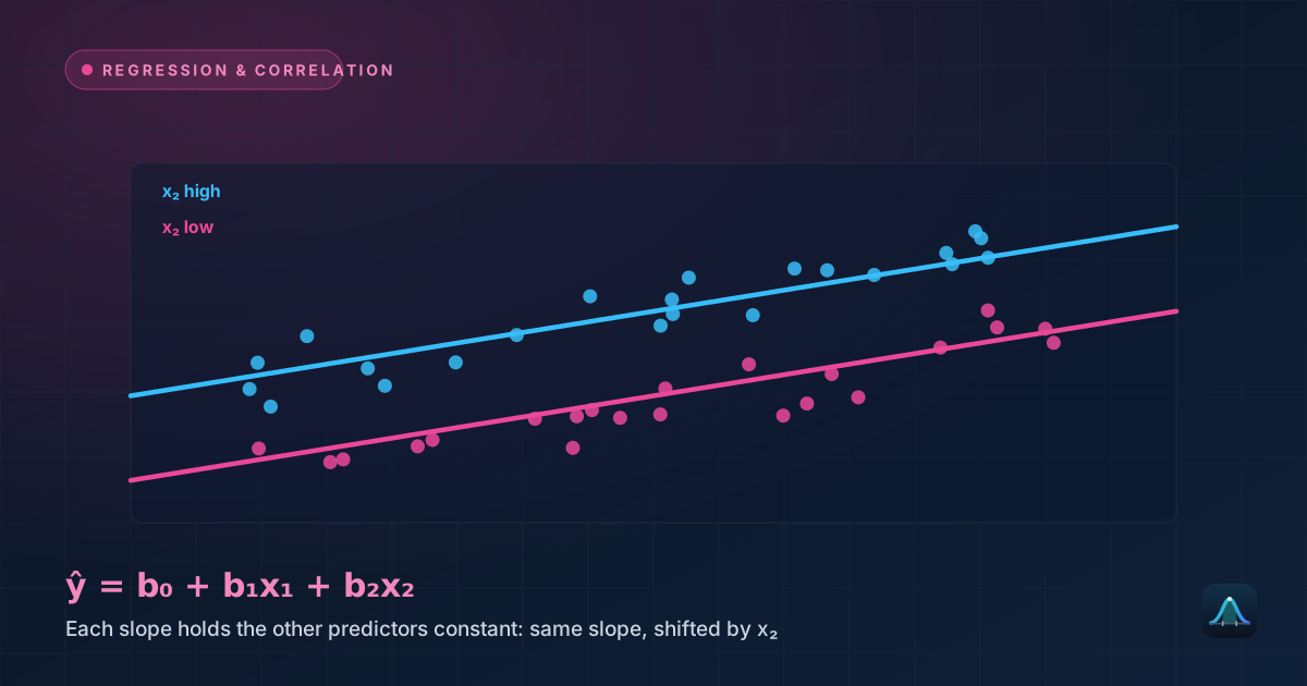
Partial correlation is the conceptual bridge between simple two-variable correlation and full multiple linear regression: a multiple regression coefficient is, in essence, already answering a very similar question — the relationship between one predictor and the outcome, holding the other predictors constant. Partial correlation makes that same "holding constant" logic available as a standalone, simpler calculation, useful specifically when the goal is quantifying a relationship's strength after removing a confound, without needing to build a full regression model.

Real-World Uses

Medical research: studying the relationship between two health outcomes while controlling for age is one of the most common applications — age tends to correlate with nearly everything, and failing to control for it is a routine source of misleading raw correlations in health data.

Economics: examining the relationship between two economic indicators (like unemployment and consumer spending) while controlling for a broader economic cycle variable helps separate a genuine direct relationship from one that's really just both variables tracking the same underlying business cycle.

Psychology and social science: testing whether a relationship between two psychological measures survives after controlling for a known confound (like socioeconomic status, or the anxiety example above) is standard practice before claiming a specific, more targeted relationship exists between the two variables of actual interest.

Common Mistakes

Assuming partial correlation always shrinks the original correlation. As the second worked example shows, controlling for a third variable can just as easily reveal a stronger relationship than the raw correlation suggested — the direction of the adjustment depends entirely on the specific signs and sizes of all three pairwise correlations involved.

Treating a large partial correlation as proof of causation. Removing one specific confounder's influence doesn't rule out other, unmeasured confounders still distorting the remaining relationship — partial correlation is a genuine improvement over raw correlation, not a complete solution to the correlation-versus-causation problem, and the same causal caution that applies to ordinary correlation still applies here.